Bloch Equation

The Bloch Equation, named after physicist Felix Bloch who won the Nobel Prize for discovery of magnetic resonance phenomena, describes almost all behavior seen in MRI. Here, we will describe this equation and derive key results to use for explaining the behavior of the net magnetization and its interaction with magnetic fields.

% setup MRI-education-resources path and requirements
cd ../
startup

warning: using the gnuplot graphics toolkit is discouraged

The gnuplot graphics toolkit is not actively maintained and has a number
of limitations that are ulikely to be fixed.  Communication with gnuplot
uses a one-directional pipe and limited information is passed back to the
Octave interpreter so most changes made interactively in the plot window
will not be reflected in the graphics properties managed by Octave.  For
example, if the plot window is closed with a mouse click, Octave will not
be notified and will not update it's internal list of open figure windows.
We recommend using the qt toolkit instead.

loading image
loading signal

Learning Goals

1. Understand what MRI is measuring

   • Understand what the net magnetization is

2. Describe the concepts of polarization, resonance, and relaxation

   • Describe the rotation of the net magnetization in response to magnetic fields

   • Describe the process of relaxation

THE Bloch Equation

The Bloch equation describes the behavior of the net magnetization, \(\vec{M}(\vec{r},t)\), in a magnetic field, \(\vec{B}(\vec{r},t)\), and can describe the vast majority of all MRI phenomena. While the complete Bloch Equation is presented here, we can typically use results derived from this equation to analyze and design MRI experiments.

\[\begin{split} \frac{d\vec{M}(\vec{r},t)}{dt} = \gamma \vec{M}(\vec{r},t) \times \vec{B}(\vec{r},t) + \begin{bmatrix} -1/T_2(\vec{r})& 0 & 0 \\ 0 & -1/T_2(\vec{r}) & 0 \\ 0 & 0 & -1/T_1(\vec{r}) \end{bmatrix} \vec{M}(\vec{r},t) + \begin{bmatrix} 0 \\ 0 \\ M_0(\vec{r})/T_1(\vec{r}) \end{bmatrix} \end{split}\]

The beavhior depends on constants of:

• \(M_0(\vec{r})\) - the equilibrium magnetization

• \(T_1(\vec{r})\) - the longitudinal (\(M_Z\)) or spin-lattice relaxation time constant

• \(T_2(\vec{r})\) - the transverse (\(M_{XY}\)) or spin-spin relaxation time constant

All of which can vary across our subject (and all a valuable source of contrast!).

There is a very full-featured, interactive Bloch Equation Simulator available online, that is valuable to understand the behavior of the net magnetization:
Bloch Equation Simulator

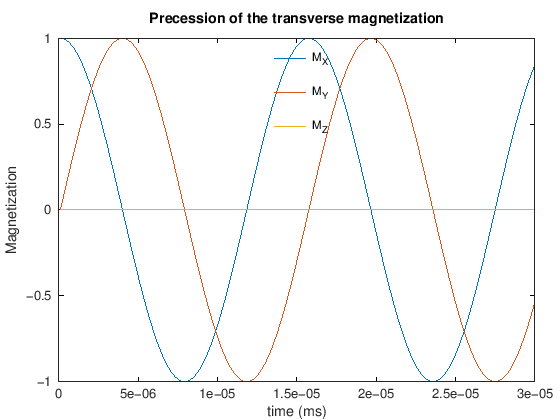
Precession

The first term in the Bloch equation means that the net magnetization, \(\vec{M}\) rotates around the magnetic field, \(\vec{B}\), with a left-handed rotation. This rotation is sometimes referred to as precession.

To observe this, we neglect relaxation (\(T_1, T_2 \rightarrow \infty\)):

\[ \frac{d\vec{M}(t)}{dt} = \gamma \vec{M}(t) \times \vec{B}(t) \]

Simulation of Precession

Open up the Bloch Equation Simulator. You will see a visualization of a net magnetization vector that is precessing around the magnetic field (thin line).

B0 = 1.5e3; % 1.5 T = 1500 mT
% using units of mT and ms for the bloch_rotate function

% start at equilibrium
Mstart = [0,0,1].'; 
% after RF excitation
Mstart = [1,0,0].'; 


Bstatic = [0,0,B0];

% animate rotation?
dt = .1e-6; % .1 ns = .1e-6 ms
N = 300;
t = [1:N]*dt;
Mall = zeros(3,N);
Mall(:,1) = Mstart;
for It = 1:N-1
    Mall(:,It+1) = bloch_rotate(Mall(:,It),dt,Bstatic);
end

plot(t,Mall)
xlabel('time (ms)'), ylabel('Magnetization')
legend({'M_X', 'M_Y', 'M_Z'}, 'location', 'north'), legend boxoff
title(['Precession of the transverse magnetization'])

ans = -9.5540
ans = -9.5540

RF Excitation

RF excitation occurs when an oscillating magnetic field is applied orthogonally to the main magnetic field. If we apply RF at the Larmor frequency, the magnetic field would be

\[\begin{split}\vec{B}(\vec{r},t) = \begin{bmatrix} B_{1}^+(\vec{r},t) \cos(2\pi\bar{\gamma} B_0 t) \\ B_{1}^+(\vec{r},t) \sin(2\pi\bar{\gamma} B_0 t) \\ B_0 \end{bmatrix}\end{split}\]

When applied at the Larmor frequency, the applied RF energy and the net magnetization are in resonance, and we achieve excitation.

Example: Constant amplitude pulse

A good first RF excitation pulse to consider is a constant amplitude RF pulse, \(B_{1}^+(\vec{r},t) = B_{1,0}\). When this is applied on resonance, the Bloch equation results in a progressive rotation of the net magnetization away from the z-axis, as illustrated below:

Lab versus Rotating Frame

For simplification, we use the so-called “rotating frame” - a reference frame that is rotating around the main field (z-axis) at the Larmor frequency, \(f_0 = \bar{\gamma} B_0\), which greatly simplifies the interpretation, visualization, and math when analyzing the Bloch equation. This is in contrast to the “lab frame” or “stationary frame”.

In the rotating frame, the magnetic field vector is transformed to both have the rotation of the RF pulse terms removed. In this transformation of reference frames, the main magnetic field, \(B_0\), is also removed. This change in the representation removes the precession of \(\vec{M}\) around the z-axis, as we should expect in the rotating frame.

\[\begin{split}\vec{B}(t) = \begin{bmatrix} B_{1,X}^+(\vec{r},t) \\ B_{1,Y}^+(\vec{r},t) \\ 0 \end{bmatrix}\end{split}\]

Now we can analyze RF excitation as a rotation around RF magnetic field amplitude and do not have to include Larmor frequency in our analysis, shown in the illustration below:

Common flip angle RF excitations

For a constant amplitude RF pulse, the flip angle depends on the duration of the RF pulse, \(T_{rf}\) and the strength of the RF magnetic field, \(b_{1,0}\):

\[\theta = \gamma b_{1,0} T_{rf} \]

45-degree flip	90-degree flip	180-degree flip

Simulations of RF Excitation

Again, open up the Bloch Equation Simulator.

1. Lab versus rotating frame: The default view is in the lab (stationary) frame. If you select the ‘B0’ option from the ‘Frame’ in the top left it will change to the rotating frame.

2. RF Excitation: Change to ‘Equilibrium’ scene in bottom left. Then, use the ‘90x hard’ button to apply a constant amplitude pulse.

3. Other flip angles: Go back to ‘Equilibrium’ scene, and try the other hard RF pulse flip angles.

Below are additional Bloch equation simulations and associated code for RF excitation show non-resonant magnetic fields, resonant magnetic fields, and excitation in the rotating frame.

First, when a non-resonant magnetic field is applied. An additional magnetic field is applied orthogonal to the main magnetic field, but not applied at the Larmor frequency, and there is no creation of transverse magnetization.

% lab frame

gammabar = 42.58; % kHz/mT

B0 = 10; %  10 mT for simplicity to visualize rotation
f0 = gammabar*B0 % kHz

M0 = 1;
M_equilibrium = [0,0,M0].';

% RF pulse paarameters
T_RF =  1; % ms
t = linspace(0, T_RF, 4000);

RF_flip_angle = pi/2; % radians
B10 = RF_flip_angle / (2*pi*gammabar*T_RF) % mT

f0 = 425.80

B10 = 5.8713e-03

% RF not applied at resonance frequency (constant magnetic field in X)
% lab frame
B = [B10;0;B0];  

Mall = zeros(3,length(t));
Mall(:,1) = M_equilibrium;
for It = 1:length(t)-1
    Mall(:,It+1) = bloch_rotate(Mall(:,It),t(It+1) - t(It),B);
end

plot(t,Mall)
xlabel('time (ms)'), ylabel('Magnetization')
legend({'M_X', 'M_Y', 'M_Z'}, 'location', 'north'), legend boxoff
title(['Non-resonant magnetic field (in RF direction)'])

ans = -12.513
ans = -12.513

To achieve excitation the RF pulse is applied at the Larmor frequency, \(\omega_0 = \gamma B_0\). With a resonant RF pulse, we have excitation of the net magnetization away from the direction of the main magnetic field, and creation of transverse magnetization, \(M_X\) and \(M_Y\).

% RF pulse at Larmor frequency
% lab frame
B = [B10*cos(2*pi*f0*t);B10*-sin(2*pi*f0*t);B0*ones(1,length(t))];  

Mall = zeros(3,length(t));
Mall(:,1) = M_equilibrium;
for It = 1:length(t)-1
    Mall(:,It+1) = bloch_rotate(Mall(:,It),t(It+1) - t(It),B(:,It));
end

plot(t,Mall)
xlabel('time (ms)'), ylabel('Magnetization')
legend({'M_X', 'M_Y', 'M_Z'}, 'location', 'northwest'), legend boxoff
title(['Resonant RF pulse'])

ans = -12.192
ans = -12.192

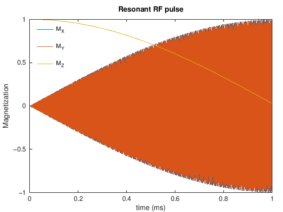
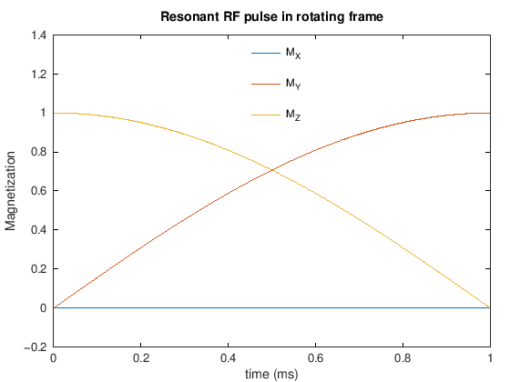
Finally, the simulation is converted into the rotating frame. It is hard to visualize the transverse magnetization in the lab because it is rotating at the Larmor frequency. The excitation is more clearly visualized in the rotating frame.

% rotating frame
% RF pulse at Larmor frequency
B = [B10;0;0];  

Mall = zeros(3,length(t));
Mall(:,1) = M_equilibrium;
for It = 1:length(t)-1
    Mall(:,It+1) = bloch_rotate(Mall(:,It),t(It+1) - t(It),B);
end

plot(t,Mall)
xlabel('time (ms)'), ylabel('Magnetization')
legend({'M_X', 'M_Y', 'M_Z'}, 'location', 'north'), legend boxoff
title(['Resonant RF pulse in rotating frame'])

ans = -12.438
ans = -12.438

Relaxation

The other key result of the Bloch equation is that the net magnetization will return to equilibriuam over time with specific time constants, called \(T_1\) and \(T_2\). More specifically relaxation depends on

• \(M_0(\vec{r})\) - the equilibrium magnetization, where the magnetic field ultimately is oriented in the same direction as the main magnetic field along the z-axis as: \(\vec{M}(\vec{r}, t \rightarrow \infty) = [0, 0, M_0(\vec{r})]^T\)

• \(T_1(\vec{r})\) - the longitudinal (\(M_Z\)) or spin-lattice relaxation time constant

• \(T_2(\vec{r})\) - the transverse (\(M_{XY}\)) or spin-spin relaxation time constant

In the rotating frame, without any applied RF energy, the Bloch equation is simplified to

\[\begin{split} \frac{d\vec{M}(t)}{dt} = \begin{bmatrix} -1/T_2& 0 & 0 \\ 0 & -1/T_2 & 0 \\ 0 & 0 & -1/T_1 \end{bmatrix} \vec{M}(t) + \begin{bmatrix} 0 \\ 0 \\ M_0/T_1 \end{bmatrix} \end{split}\]

This has solutions of

\[\begin{split} \vec{M}(t) = \begin{bmatrix} e^{-t/T_2} & 0 & 0 \\ 0 & e^{-t/T_2} & 0 \\ 0 & 0 & e^{-t/T_1} \end{bmatrix} \vec{M}(0) + \begin{bmatrix} 0 \\ 0 \\ M_0(1-e^{-t/T_1}) \end{bmatrix} \end{split}\]

or

\[M_{XY}(t) = M_{XY}(0) e^{-t/T_2}\]

\[M_Z(t) = M_Z(0)e^{-t/T_1} + M_0(1- e^{-t/T_1})\]

Where here the shorthand complex notation for the transverse magnetization is being used: \(M_{XY}(\vec{r},t) = M_X(\vec{r},t) + i M_Y(\vec{r},t)\)

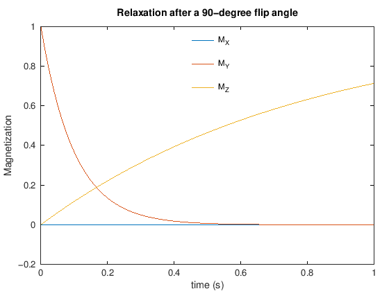
T1 and T2 relaxation after RF Excitation

Simulation of Relaxation

One more time, open up the Bloch Equation Simulator. Under the ‘Relaxation’ options in the top left, you can adjust T1 and T2 relaxation rates.

1. Experiment with different T1 and T2 relaxation values

2. When the magnetization turns to equilibrium, use a RF pulse and you will see relaxation occurring again.

3. From Equilibrium, try a 180-degree flip angle and try adjusting both T1 and T2. Which parameter influence the relaxation in this situation?

Below are additional Bloch equation simulations and associated code of relaxation.

t = linspace(0,1); % s

M0=1;
T1 = .8;  T2 = .1; % s
M_equilibrium = [0,0,M0].';

flip= 90;

gammabar = 42.58; % kHz/mT
T = 1; % 1 ms pulse duration
% calculate RF pulse amplitude (milliTesla)
B10 = flip*pi/180 / (2*pi*gammabar*T)

% apply RF tip
M_start = bloch_rftip(M_equilibrium, T, B10)

Mall = zeros(3,length(t));

for It = 1:length(t)
    Mall(:,It) = bloch_relax(M_start,t(It),M0,T1, T2);
end

B10 = 5.8713e-03

M_start =

  -6.1232e-17
   1.0000e+00
   6.1232e-17

plot(t,Mall)
xlabel('time (s)'), ylabel('Magnetization')
legend({'M_X', 'M_Y', 'M_Z'}, 'location', 'north'), legend boxoff
title(['Relaxation after a ' num2str(flip) '-degree flip angle'])

ans = -12.657
ans = -12.657