Spectral-Spatial RF Pulses

Spectral-spatial RF pulses aim to provide both

• spectral selection, typically to only excite protons in water molecules, and not protons in lipids

• spatial selection, for slice-selective imaging

These are particularly common in fMRI and diffusion with echo-planar imaging (EPI) in order to eliminate chemical shift displacement artifacts in the image, and are also used for water and/or fat suppression in MR spectroscopy.

Learning Goals

1. Describe how images are formed

   • Understand how spectral-spatial RF pulses work

2. Identify artifacts and how to mitigate them

   • Determine when using spectral-spatial RF pulses would help remove chemical shift related artifacts

Spectral-Spatial RF Pulse Design

This is done by creating a 2D excitation profile in both the spectral and spatial dimensions. This is most easily interpreted through excitation k-space, where the RF energy deposited can be Fourier Transformed to reveal the approximate spectral-spatial profile created.

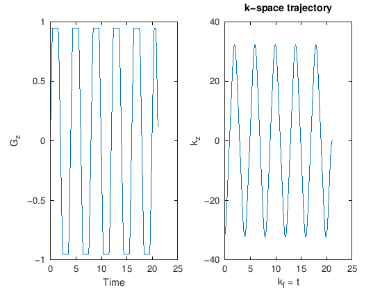
The gradient applied traverses spatial excitation k-space, while time traverses the spectral excitation k-space dimension, as demonstrated by the gradient and k-psace plot below

% setup MRI-education-resources path and requirements
cd ../
startup

% trick to compile abr() mex file
abr([1 1], [0 0], 0);

warning: using the gnuplot graphics toolkit is discouraged

The gnuplot graphics toolkit is not actively maintained and has a number
of limitations that are ulikely to be fixed.  Communication with gnuplot
uses a one-directional pipe and limited information is passed back to the
Octave interpreter so most changes made interactively in the plot window
will not be reflected in the graphics properties managed by Octave.  For
example, if the plot window is closed with a mouse click, Octave will not
be notified and will not update it's internal list of open figure windows.
We recommend using the qt toolkit instead.

loading image
loading signal

error: MEX file now compiled, re-run code
error: called from
    abrx at line 31 column 1
    abr at line 31 column 12

% Demonstrate gradient and spectral-spatial k-space trajectoy

GAMMA = 42.58;
dt = 0.1;

Nlobe = 20;
Nspec = 10;
Nramp = 4;

ramp = [.5:Nramp-.5]/Nramp;
g1 = [ramp, ones(1,Nlobe-2*Nramp), ramp(end:-1:1)]; 

gamp = 0.95;
g = [];
for k = 1:Nspec
   g = [g, (mod(k,2)*2 - 1)*gamp*g1];
end

Nrw = round((Nlobe - Nramp)/2 + Nramp);
grw = [ramp, ones(1,Nrw-2*Nramp), ramp(end:-1:1)];

g = [g, (mod(Nspec+1,2)*2-1)*gamp*grw];

t = [0:length(g)-1]*dt;
subplot(121)
plot(t, g)
ylabel('G_z')
xlabel('Time')

subplot(122)
plot(t, GAMMA*dt*(cumsum(g) - sum(g)))
xlabel('k_f = t'), ylabel('k_z')
title('k-space trajectory')

To design the RF pulse, we can approximate the pulse and profile shape as separable function in frequency and space:

\[ h(f,z) = h_f(f) h_z(z)\]

\[ \mathcal{F}\{ h(f,z) \} = H(k_f, k_z) = H_f(k_f) H_z(k_z)\]

With this approximation, we can formulate the goal of the RF pulse design is to create and combine two pulses:

• A spectral pulse filter, \(H_f(k_f)\), that should be applied in \(k_f\) direction

• A spatial pulse filter, \(H_z(k_z)\), that should be applied in the \(k_z\) direction

Then design typically consists of 3 main steps

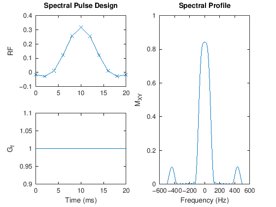
1. Design spectral pulse (envelope)

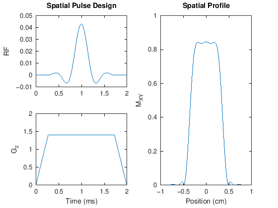
2. Design spatial sub-pulse

3. Combine spectral pulse envelope and spatial subpulses with an oscillating gradient

% Design parameters
GAMMA = 4258; % Hz/G
slewmax = 15e3; % G/cm/s
gmax = 4; % G/cm
T = 20e-3; % ms
TBW = 3;
SBW = 6;
dz = 0.5; % cm, max spatial resolution
Nspec = 10;
DT = T/Nspec;
dt = 10e-6; % us
flip = pi/4;

% gradient parameters
verse_frac = 0.8;
Nlobe = DT/dt;
Nspat = round(Nlobe * verse_frac);
Nwait = (Nlobe - Nspat)/2;

z = linspace(-0.8, 0.8, 201);
df = linspace(-500, 500, 201);

% 1. Spectral Pulse Design

rfspec = dzrf(Nspec, TBW);
gf = 2*pi*DT * ones(1,length(rfspec));
mxy_f = ab2ex(abr(rfspec, gf, df));

t = [0:length(rfspec)-1]*DT*1e3;
subplot(221)
plot(t, real(rfspec), '-x')
ylabel('RF')
title('Spectral Pulse Design')
subplot(223)
plot(t, ones(1,length(rfspec)))
ylabel('G_f')
xlabel('Time (ms)')
subplot(122)
plot(df, abs(mxy_f))
xlabel('Frequency (Hz)'), ylabel('M_{XY}')
title('Spectral Profile')

% 2. Spatial pulse design

rfspat = dzrf(Nspat, SBW);

% gradients (including ramp sampling)
gamp = (SBW/DT)/(GAMMA*dz); % gradient for spatial resolution

% Uses a slew rate that can't be violated
Nramp = min( ceil(gmax/slewmax / dt), floor(Nlobe/2));
ramp = [.5:Nramp-.5]/Nramp;
g1 = [ramp, ones(1,Nlobe-2*Nramp), ramp(end:-1:1)]; 
% apply VERSE algorithm for time-varying gradient
rfspatv = verse(g1, [zeros(1, floor(Nwait)), rfspat(:).', zeros(1,ceil(Nwait))]).';
rfspatv(find(isnan(rfspatv))) = 0;

g1z = 2*pi*GAMMA*dt * gamp* g1;
mxy_z = ab2ex(abr(rfspatv, g1z, z));

t = [0:length(g1)-1]*dt*1e3;
subplot(221)
plot(t, real(rfspatv))
ylabel('RF')
title('Spatial Pulse Design')

subplot(223)
plot(t, gamp*g1)
ylabel('G_z')
xlabel('Time (ms)')

subplot(122)
plot(z, abs(mxy_z))
xlabel('Position (cm)'), ylabel('M_{XY}')
title('Spatial Profile')

% 3. Combine spectral and spatial pulse designs

rf = []; g = [];
for k = 1:Nspec
   rf = [rf, rfspatv*rfspec(k)];  % weight spatial sub-pulses by the spectral filter
   g = [g, (mod(k,2)*2 - 1)*gamp*g1];  % oscillate gradient
end

% add spatial refocusing gradient
Nrw = round((Nlobe - Nramp)/2 + Nramp);
grw = [ramp, ones(1,Nrw-2*Nramp), ramp(end:-1:1)];

g = [g, (mod(Nspec+1,2)*2-1)*gamp*grw];
rf = [rf, zeros(1,Nrw)];

% scale RF pulse
flip_scale = flip/sum(rf);
rf = flip_scale*rf;
rfs = rfscaleg(rf, T);

figure
subplot(211)
plot([0:length(rf)-1]*dt*1e3, real(rf), ...
    [0.5:1:length(rfspec)-0.5]*DT*1e3, real(rfspec)/max(real(rfspec)) * max(real(rf)), '--')
    legend('RF pulse', 'Spectral pulse envelope')
ylabel('RF')
title('Spectral-Spatial RF Pulse')
subplot(212)
plot([0:length(rf)-1]*dt*1e3, g)
ylabel('G_z')
xlabel('Time (ms)')

figure
plot3([-length(rf)+1:0]*dt*1e3, GAMMA*dt*(cumsum(g) - sum(g)), real(rf))
xlabel('k_f = t'), ylabel('k_z')
title('B_1(k)')

ans = -11.589

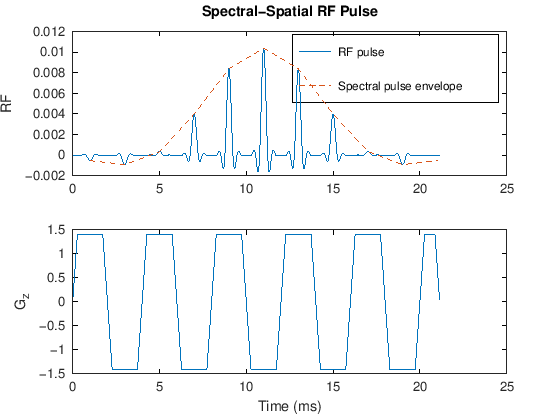
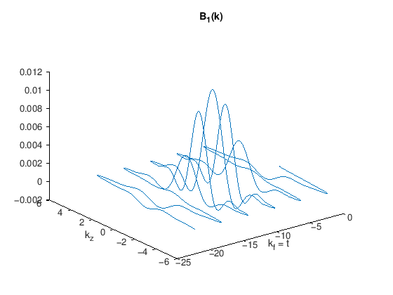
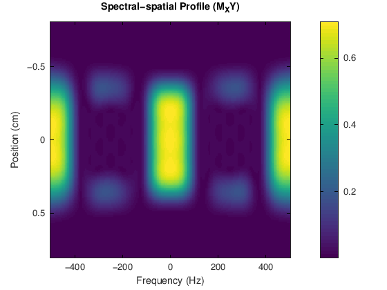
The spectral pulse, \(H_f(k_f)\), creates the overall envelope, and is applied as a weighting for repeated versions of the spatial pulse, \(H_z(k_z)\). This creates the excitation k-space profile, \(B_1(k_f, k_z)\) shown above, which results in the spectral-spatial profile shown below:

gz = 2*pi*GAMMA*dt * g;
gf = 2*pi*dt * ones(1,length(rf));

mxy_2d = ab2ex(abr(rf, gz + i*gf, z, df));


figure
imagesc(df,z,abs(mxy_2d))
xlabel('Frequency (Hz)'), ylabel('Position (cm)')
title('Spectral-spatial Profile (M_XY)')
%colormap(gray)
colorbar

Watch how the transverse magnetization evolves during the spectral-spatial RF pulse: