Cartesian Sampling Image Characteristics#
The most common type of pulse sequence uses Cartesian sampling on a k-space grid using frequency and phase encoding. Here we explicitly define the image characteristics of FOV, resolution, scan time, and SNR for this sequence.
Learning Goals#
Describe how images are formed
Determine the image FOV and resolution when using Cartesian sampling
Determine the scan time when using Cartesian sampling
Manipulate MRI sequence parameters to improve performance
Determine how Cartesian sequence parameters will change FOV and resolution
Determine how changes in sequence parameters will affect the scan time and SNR
Cartesian Pulse Sequence#
The following pulse sequence diagram shows a Cartesian 2D FT sequence including relevant pulse amplitudes and durations needed to determine the image characteristics. A gradient-echo sequence is shown, and the principles can simply be extended to a spin-echo sequence.
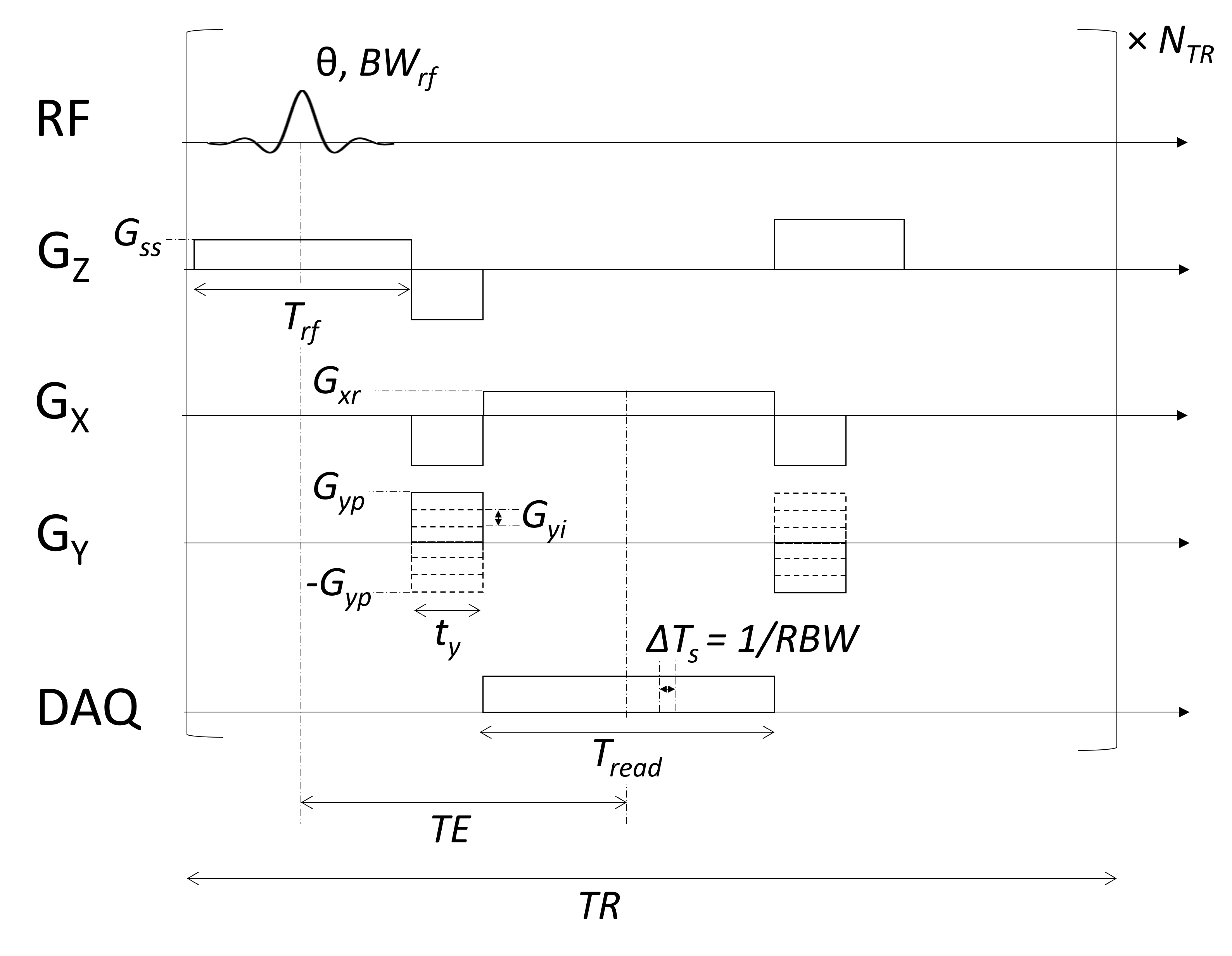
Note that idealized rectangular gradients are shown for simplicity.
Spatial Resolution#
The spatial resolution is determined by the maximum sample extent in k-space. In the frequency encoding, this can be calculated from the total gradient area during the readout:
In the phase encoding, we can calculate the maximum k-space extent bassed on the largest phase encoding gradient area:
In the slice select dimension, the spatial resolution is determined by the slice thickness:
Field-of-View (FOV)#
The FOV is determined by the sample spacing in k-space. In the frequency encoding, this is determined by the sampling rate or the readout bandwidth, \(\Delta T_s = 1/RBW\) and the gradient area during that time:
In the phase encoding, this is determined by the difference in gradient area between adjacent phase encoding steps:
All of these relationships can also be rewritten using the relationship between FOV, resolution, and number of voxels.
where \(N_{FE}\) is the number of samples in the frequency encoding direction and \(N_{PE}\) is the number of samples in the phase encoding direction.
Scan Time#
For this sequence, the total scan time is determined by the TR and the number of TRs, \(N_{TR}\):
Assuming no acceleration, the number of TRs is equal to the number of phase encoding steps, \(N_{PE}\), times the number of averages, \(N_{avg}\):
SNR#
The SNR can be written for this sequence in numerous ways using the above relationships. This is left as an exercise to the reader.