The Pulse Sequence

Magnetic resonance experiments are described by a “Pulse Sequence”, which is a timing diagram that shows how the different magnetic fields are manipulated. This chapter introduces the pulse sequence diagram and the sequence parameters of TE and TR.

Learning Goals

1. Understand what MRI is measuring

   • Identify when signals are measured during a MRI experiment

2. Describe how various types of MRI contrast are created

   • Understand what is shown in a pulse sequence diagram

3. Describe how images are formed

   • Understand that a pulse sequence must be repeated to form an image

Components of a Pulse Sequence

All MRI experiments can be defined by their pulse sequence. This describes all manipulations of the MRI scanner being done, including their relative timings and amplitudes.

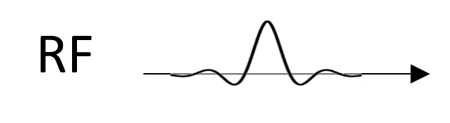
RF Excitation pulse (RF)

The RF excitation pulse is the first required component, as it rotates or flips the magnetization into the transverse plane, creating resonance of the net magnetization that can actually be measured.

Magnetic field gradients for localization (\(G_X, G_Y, G_Z\))

The magnetic field gradients are also used in a pulsed fashion, where they are switched on and off during the pulse sequence. This is done primarily for spatial localization, including RF pulse slice selection and spatial encoding, which are both described in later chapters. It is important to note here that multiple measurements with slightly different gradient pulses must typically be used to get enough data to form an image.

Data acquisition window (DAQ)

The data acquisition window indicates when signals are being measured and recorded off of the RF receive coils. This must be done after excitation, and is done in conjunction with magnetic field gradients to perform spatial encoding. It is important to remeber when looking at the data acquisition window that it is the transverse magnetization (\(M_{XY}\)) that is measured.

Pulse Sequence Diagrams

The pulse sequence diagram is an incredible tool for conveying a significant amount of information about a MRI experimental method. It can capture the expected image contrast, the type of spatial encoding, the overall imaging speed, and more.

Sample Pulse Sequence Diagram

The pulse sequence diagram has lines for each component (RF pulses; magnetic field gradients in X, Y, and Z; data acquisition) to show their behavior over time. A single “block” of the sequence is usually shown, but this block is usually repeated many times (see below).

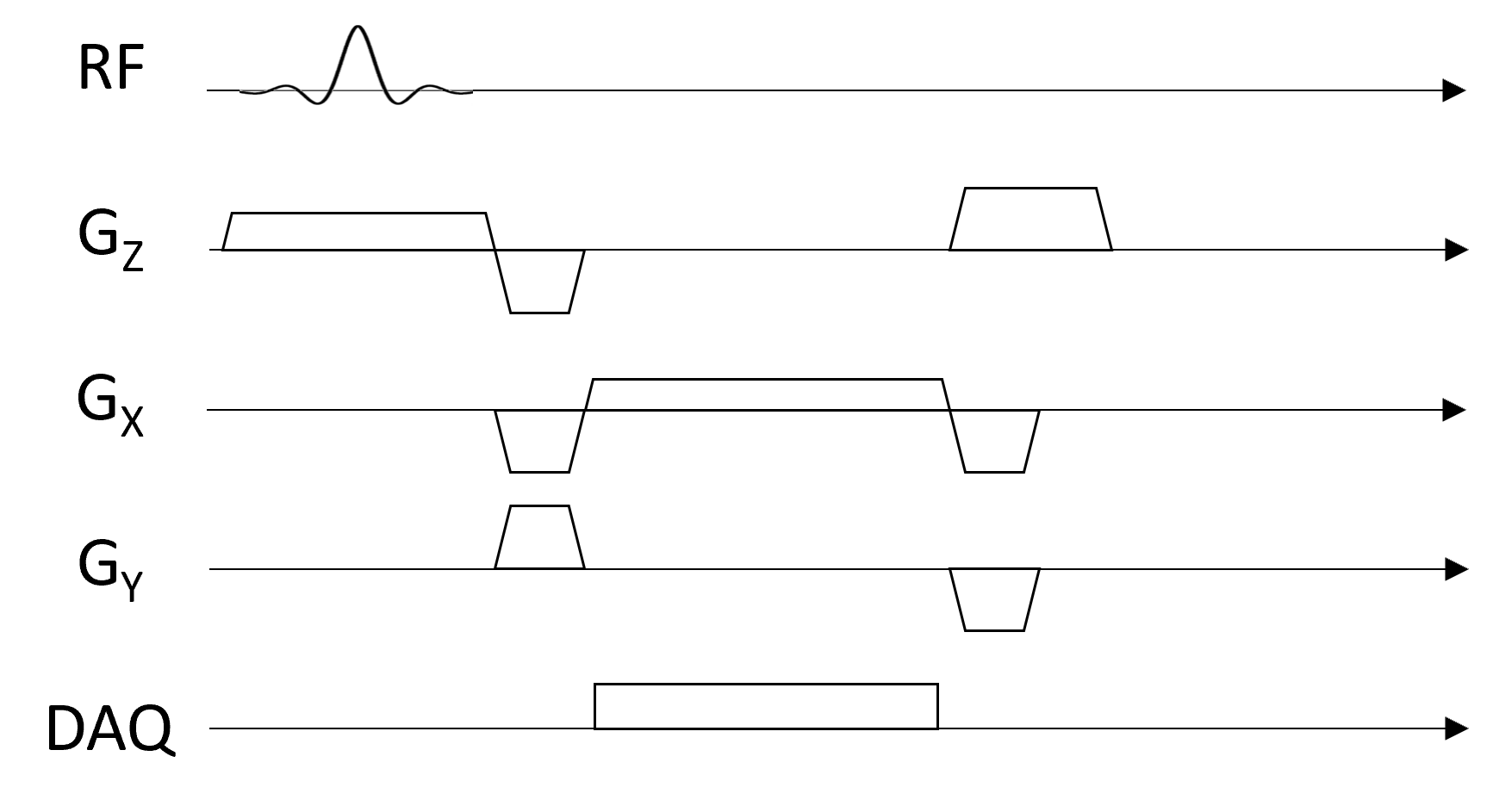
Note that the RF pulses as drawn to not show that these pulses are actually applied at very high frequencies near Larmor resonance frequency.

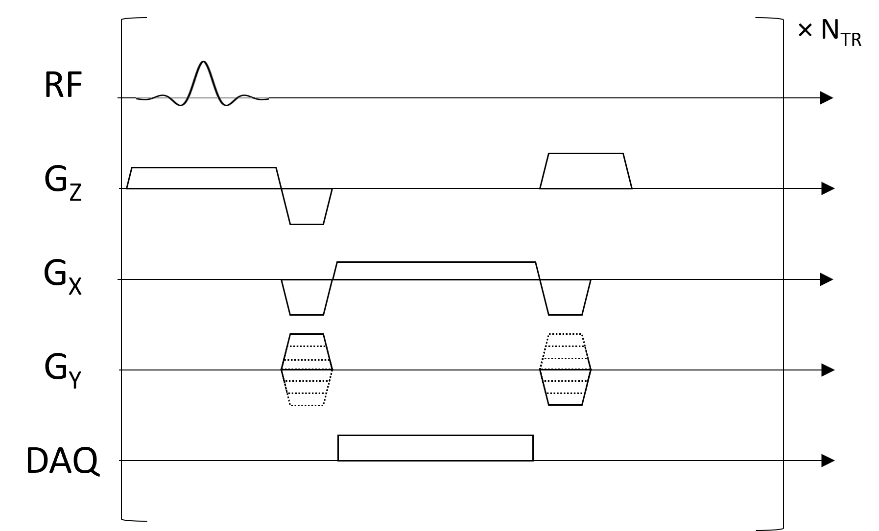
Annotations

In most every MRI experiment, the basic pulse sequence block is repeated but with a different gradient pattern to perform the necessary spatial encoding. This is typically annotated in 2 ways. First, the changes in gradient patterns can be added through multiple lines on the gradient axes. Second, bracketing around the sequence is sometimes used along with annotation that shows how many times the pulse sequence block is repeated.

Simplified diagrams

For analyzing in particular image contrast and relaxation, it is often helpful to use a simplified pulse sequence diagram that only includes RF pulses and data acquisition windows. Sometimes, simlified representation of gradients are added as well (e.g. crushers to indicate purposeful destruction of transverse magnetization).

Also, pulse sequence diagrams are often drawn with idealized gradient shapes of rectangles, indicating the magnetic field gradients are instantaneously changed. In reality, there is some minimum time required for magnetic field gradients to change, defined by their “slew rate”, which turns the rectangles into trapezoids.

Key Parameters

The following key parameters are typically defined on a pulse sequence diagram:

• Flip Angle (\(\theta\)) - how much a RF pulse flips (i.e. rotates or tips) the net magnetization

• Echo Time (TE) - the time between excitation and data acquisition, typically measured between the center of the RF excitation pulse and the data acquisition window

• Repetition Time (TR) - the time between repetitions of the main pulse sequence block

• Number of Repetitions (\(\mathrm{N}_\mathrm{TR}\)) - how many times the pulse sequence block must be repeated