Image Contrast Examples

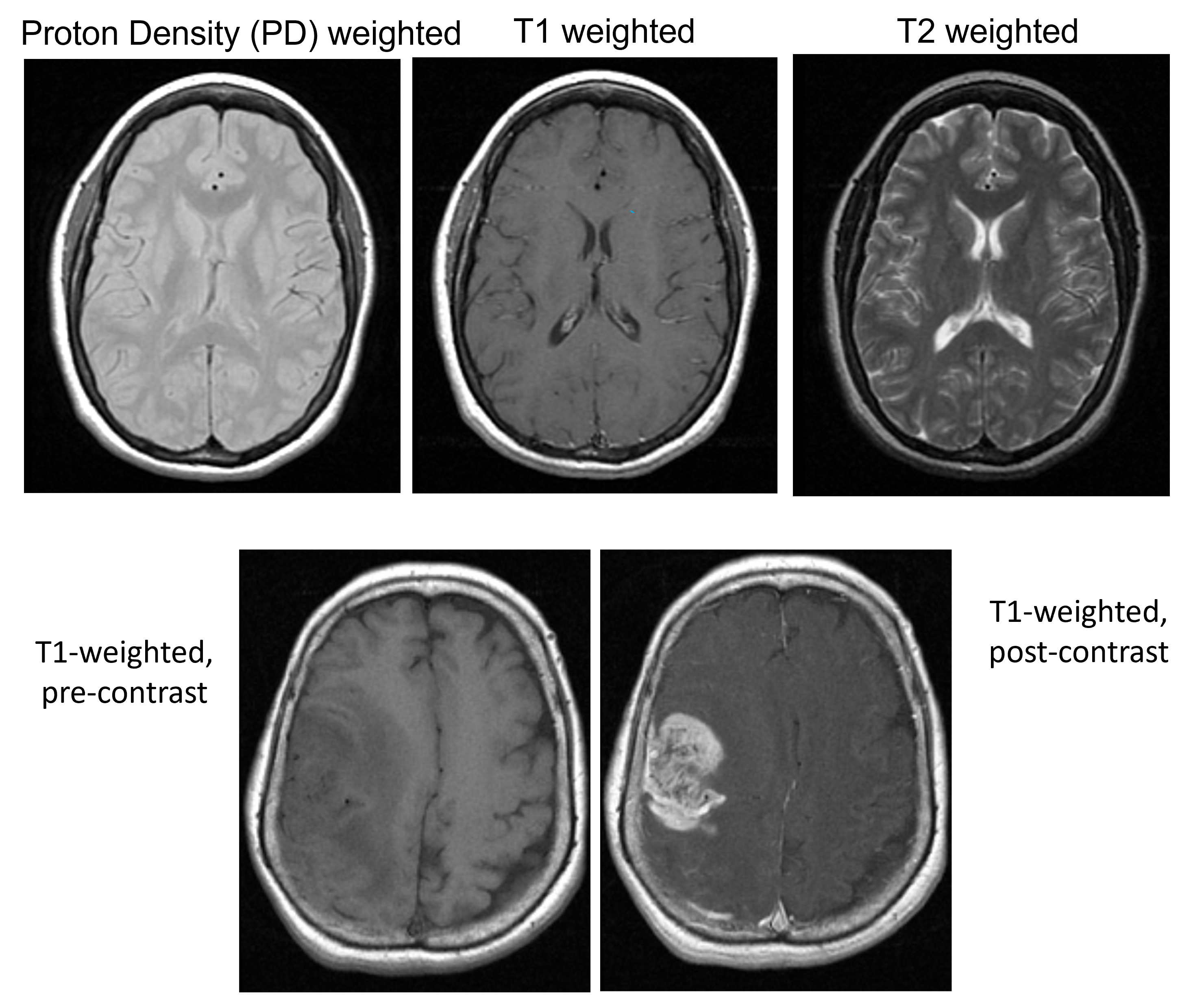
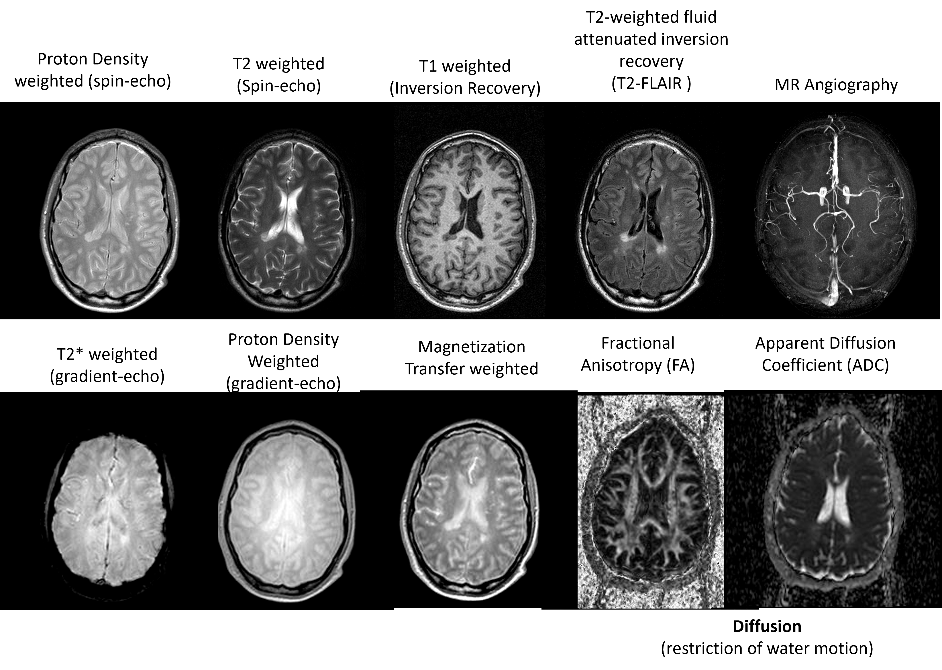
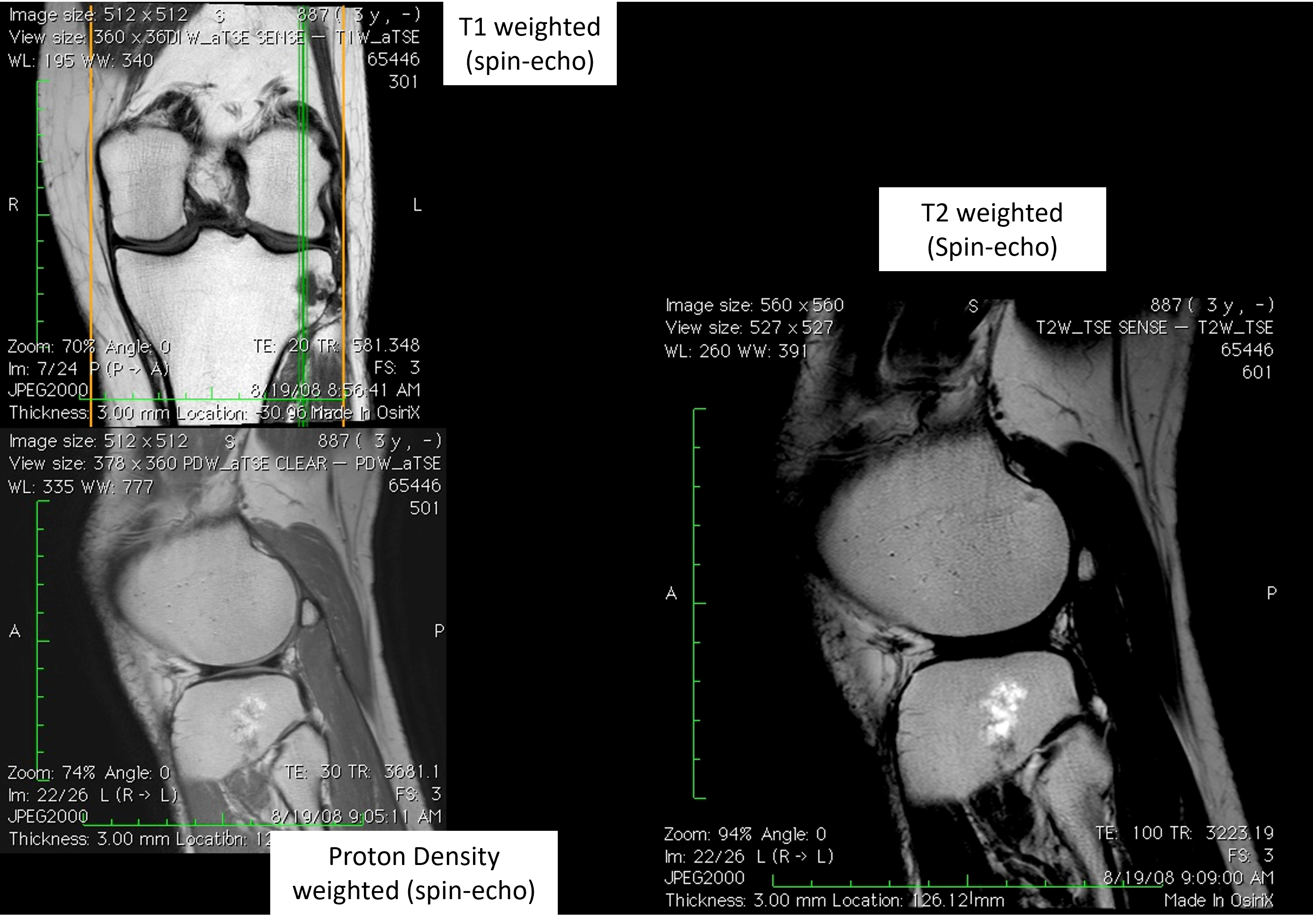
This page shows examples of different MRI contrasts, as well as examples of how to simulate MRI contrast.

Learning Goals

1. Describe how various types of MRI contrast are created

   • Identify various image contrasts

Image Contrast Examples

Simple Contrast Phantom

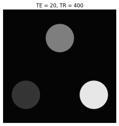
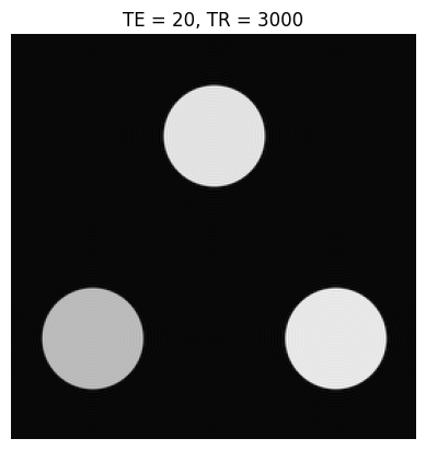
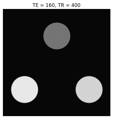
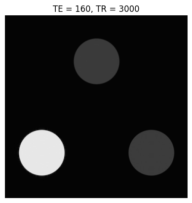
Below is a simple contrast phantom consisting of three circular objects, each with a different \(T_1\) and \(T_2\). The k-space data for these phantoms is created using a “jinc” function, which is the Fourier Transform of a circle:

\[\mathcal{F}\{ \mathrm{circ}(r) \} = \mathrm{jinc}(k_r)\]

The signal is simulated for varying sequence parameters (TE, TR) with a 90-degree flip angle in a gradient-echo scheme by using the helper function:

signal_gre = MRsignal_spoiled_gradient_echo(flip, TE, TR, M0, T1, T2)

Challenge Yourself!

Based on the images and TE/TR parameters below, can you estimate T1 and T2 relaxation times of the 3 objects?

import numpy as np
import matplotlib.pyplot as plt
from scipy.special import j1

# Helper functions (you must define these elsewhere in your notebook or import them)

def jinc(x):
    # Avoid division by zero
    result = np.ones_like(x)
    mask = x != 0
    result[mask] = j1(np.pi * x[mask]) / (2 * x[mask])
    return result

def MRsignal_spoiled_gradient_echo(flip, TE, TR, M0, T1, T2):
    # Calculate the MR signal for a spoiled gradient echo sequence
    E1 = np.exp(-TR / T1)
    E2 = np.exp(-TE / T2)
    return M0 * (1 - E1) * np.sin(flip) * E2 / (1 - E1 * np.cos(flip))

Nphan = 3
# phantom parameters
xc = np.array([-.3, 0, .3]) * 256  # x centers
yc = np.array([-.25, .25, -.25]) * 256  # y centers
M0 = np.array([1, 1, 1])  # relative proton densities
T1 = np.array([.3, .8, 3]) * 1e3  # T1 relaxation times (ms)
T2 = np.array([.06, .06, .2]) * 1e3  # T2 relaxation times (ms)
r = 1/64  # ball radius, where FOV = 1

flip = 90 * np.pi / 180
TEs = [20, 160]
TRs = [400, 3000]

N = 256

# matrices with kx, ky coordinates
kx, ky = np.meshgrid(np.arange(-N/2, N/2) / N, np.arange(-N/2, N/2) / N)

for TE in TEs:
    for TR in TRs:
        # initialize k-space data matrix
        M = np.zeros((N, N), dtype=complex)

        # Generate k-space data by adding together k-space data for each individual phantom
        for n in range(Nphan):
            # Generates data using Fourier Transform of a circle (jinc) multiplied by complex exponential to shift center location
            M = M + jinc(np.sqrt(kx**2 + ky**2) / r) * \
                np.exp(1j * 2 * np.pi * (kx * xc[n] + ky * yc[n])) * \
                MRsignal_spoiled_gradient_echo(flip, TE, TR, M0[n], T1[n], T2[n])

        # reconstruct and display ideal image
        m = np.fft.fftshift(np.fft.ifft2(np.fft.ifftshift(M)))
        plt.figure()
        plt.imshow(np.abs(m), cmap='gray', aspect='equal')
        plt.axis('off')
        plt.title(f'TE = {TE}, TR = {TR}')
        plt.show()