Volumetric Imaging#
Volumetric imaging refers to the ability to acquire images across a volume. So far we have discussed methods for a single slice. This chapter will cover the techniques of 2D multi-slice imaging and 3D imaging.
Learning Goals#
Describe how images are formed
Describe how 2D-multislice imaging works
Describe how 3D imaging works
Understand the constraints and tradeoffs in MRI
Determine what type of contrast benefits from 2D-multislice vs 3D imaging
Determine how SNR changes with 2D-multislice vs 3D imaging
Understand when either 2D-multislice or 3D imaging is preferred
2D Multi-slice Imaging#
A single slice sequence can be easily extended to acquire multiple slices. The identical sequence can be used, and only the center frequency of the RF pulse needs to be changed to move the slice location.
Interleaving#
2D multi-slice is typically done in an interleaved fashion, meaning that the acquisitions for different slices will be going on at the same time. This is done because there is often extra time within each TR, which can be used to acquire other slices. An example of interleaving is shown below:

Note that the TR for each slice is defined when each individual slice is excited, meaning this time defines the T1 recovery and contrast.
Cross-talk#
Cross-talk occurs due to the imperfect slice profiles of RF pulses. If slices are placed immediately adjacent to each other, then there is some excitation by the adjacent slice RF pulses. This can be mitigated by using higher TBW RF pulses for sharper slice profiles, or by placing gaps between slices.
3D Imaging#
True 3D imaging resolves voxels in 3 dimensions with spatial encoding gradients. In Cartesian encoding, this is done by adding a phase encoding gradient in what is normally the slice dimensions. Then, a 3D area in k-space is sampled. A slice selective RF pulse can still be used, but with a bigger slice thickness, and are sometimes referred to as “slab-selective”. In some cases, non-slice selective RF pulses are used, instead relying on the limited extent of the RF receive coil profiles to limit the FOV. A 3D FT pulse sequence is shown below:
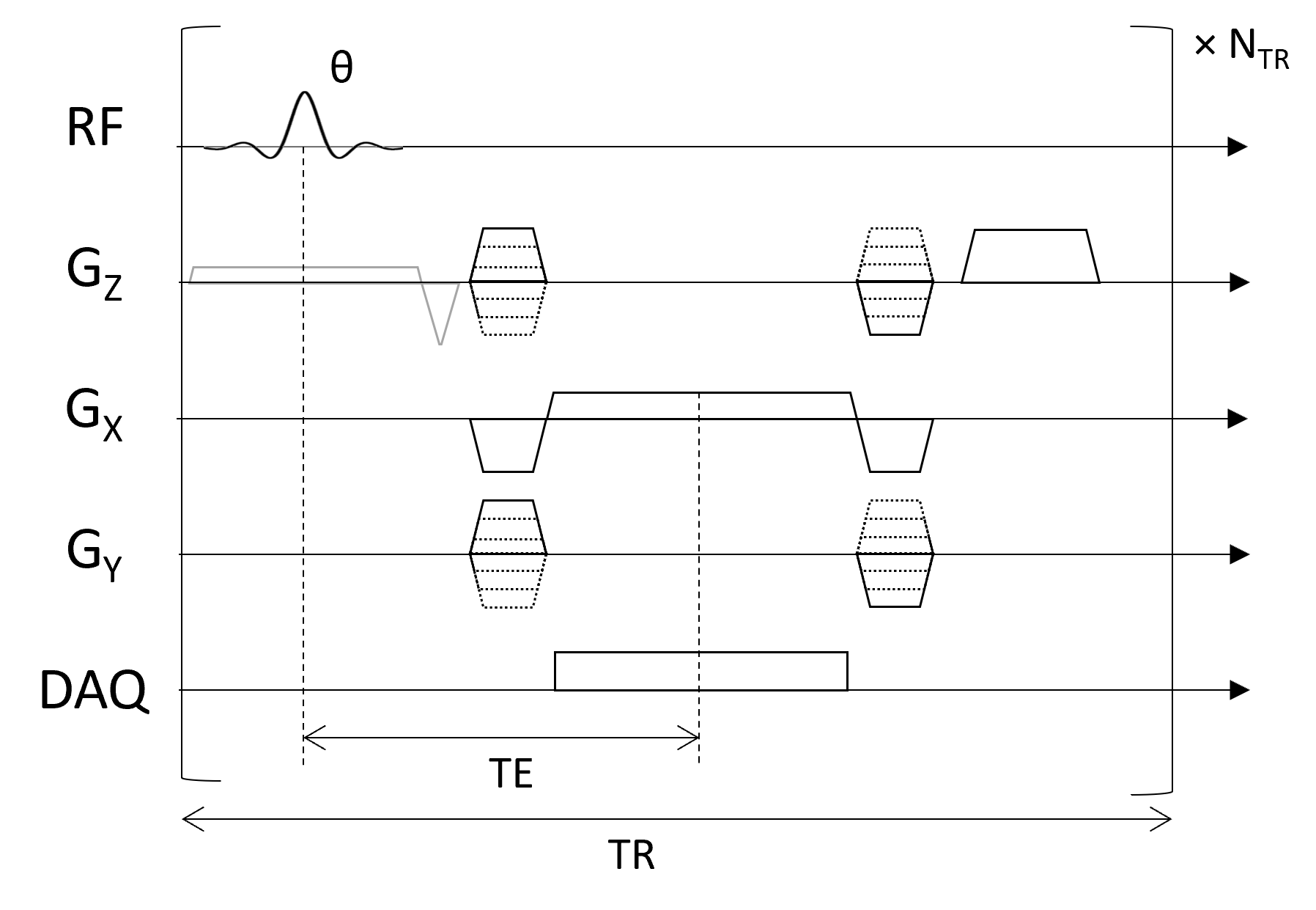
Note that now the number of TRs required is the product of the number of phase encodes in two phase encoding directions.
2D Multi-slice vs 3D Imaging#
This section outlines the tradeoffs between 2D multi-slice and 3D imaging.
Coverage#
2D multi-slice imaging can have gaps in coverage if slices are not contiguous.
3D imaging provides continuous coverages without gaps, allow for more seamless evaluation of structures.
Contrast#
2D multi-slice imaging methods with interleaving can efficiently support longer TRs for PD and T2-weighted imaging, as any extra time in the TR can be used to acquire other slices.
3D imaging methods require a larger \(N_{TR}\) to complete two dimensions of phase encoding. For this reason, they are much better suited for T1-weighted imaging which can use shorter TRs.
Scan Time#
In 2D multi-slice imaging, the scan time tradeoff depends on the number of slices that can be interleaved in a single TR. The maximum number of slices is determined by the active time:
Provided the number of slices is limited by this maximum, the scan time for fully sampled Cartesian encoding is:
In 3D imaging, the scan time depends on the size of both phase encoding dimensions:
SNR#
Here are relationships if fully-sampled Cartesian encoding is used:
3D imaging has a measurement time advantage over 2D multi-slice imaging, since each acquisition acquires signal from the entire volume. However, some of this advantage is mitigated by greater T1 recovery in 2D multi-slice imaging, which is captured by \(f_{seq}\).